Coding Lab

In the Coding or Programming Lab we develop the playbook of the modern applied and quantitatively minded economist whose ambition is to go beyond classic linear regression analysis. Many empirical research articles in the best journals feature these days a mix of economic modelling, explorative data analysis, and estimation strategies that exploit directly the structure of the initial model. The first objective of this module is to enable students to appreciate better such research designs, which requires a certain familiarity with what have become standard computational methods (such as the recursive methods of dynamic programming). Developing a working knowledge of these techniques could then lead the student to apply them in the context of their own research, in order to go beyond the constraints imposed by classic regression analysis.

We will focus first and foremost on algorithms developed in concrete economic settings (e.g. labour supply, job search), so that students can implement these in the language of their choice. For practical purposes, my illustrations are in , or Julia.

Overview: Module 1 (Introduction to Dynamic Programming and Reinforcement Learning)

Topic 1: Iterative root-finding algorithms

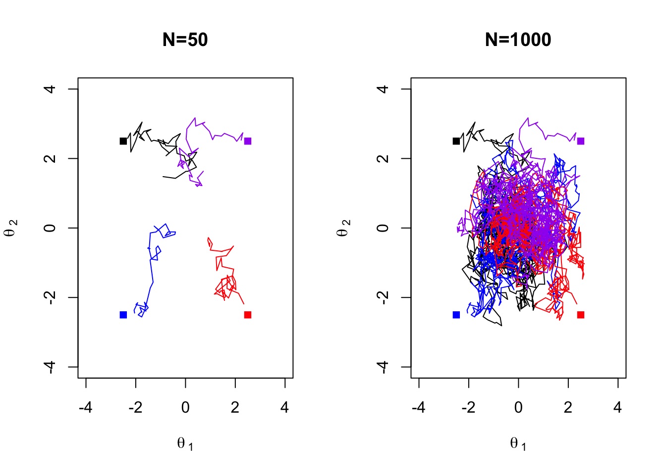
We will commence with iterative root-finding algorithms for non-linear problems, such as the Newton–Raphson method, and apply the implementation to an economic problem of static labour supply. Generically, to find the root of a univariate smooth function $f$, $f(\theta)=0$, the updating scheme is $\theta_{t+1} = \theta_t - f(\theta_t)/f’(\theta_t)$. Versions of Newton–Raphson are also used in off-the-shelf Maximum Likelihood estimation and GLMs (and their Iteratively Reweighted Least Squares implementations) such as probits in the form of so-called Fisher’s scoring or the BHHH algorithm. Generically, we have an updating scheme of the form

$$ { {\theta }} _{t+1}={ {\theta }} _{t}+\rho _{t}\mathbf {d} _{t}\left({ {\theta }}\right) $$

where $\theta$ denotes the parameter estimate, the preset $ \rho _{t}$ captures the learning rate, and $ \mathbf{d} _{t} ({{\theta }}) $ indicates the descent direction.

Several Machine Learning approaches use Gradient Descent, a closely linked updating scheme. Here the objective is to minimise a loss function $ R(\theta)$, and the scheme is $\theta _{t+1} = \theta _{t} - \rho \nabla R(\theta _{t})$ where the preset parameter $\rho$ is the learning rate and $\nabla R$ denotes the gradient of the loss function. If the data set is too large, sampling (or so-called mini-batching) leads to the Stochastic Gradient Descent method.

• [iterative schemes]
• [Static labour supply]

Topic 2: Introduction to Dynamic Programming

The second topic is dynamic optimisation, which will be done in the modern recursive way called Dynamic Programming (DP) based on the Bellman equation. For finite horizon problems, such as how to eat cake, we will proceed by backward induction. For infinite horizon problems, such as stochastic growth or search models of the labour market, we will implement
value function iterations. To speed up convergence, we will also examine policy iterations.

To be more specific (and to define the jargon), we are interested in the value function $V$ of the sequential dynamic infinite horizon optimisation problem:

$$ V (x _0) = \sup _{ {x _{t+1} } _{t=0} ^\infty } \sum _{t=0} ^\infty \beta^t F(x _t, x _{t+1}) = $$

$$
\sup_{ {x _{t+1} } _{t=0} ^\infty } F(x _0, x _1) + \beta V(x _1) $$

subject to $x_{t+1} \in \Gamma (x_t)$ for all $t \geq 0$, and $x_0$ given, where $x_t \in X$. The payoff function $F$ depends on the state variable $xt$, and $x{t+1}$ is the control variable, which also becomes the state variable in the next period. For instance, take a plain-vanilla growth model: the pay-off function is the utility function, the state variable is the current capital stock, and the consumer has to decide optimally between consumption and investment, trading-off consumption today and consumption tomorrow. In a model of job search, the searcher needs to decide whether to accept the current job offer today, or continue search in the next period.
The Bellman equation turns the sequence problem into a functional equation, $ V(s) = sup _{a \in \Gamma(s)} $ $ \left\{ F(s,a) + \beta V(s’) \right\} $. Here $s$ refers to the current state, $s’$ to the state in the next period, and $a$ to the action (choice). The right-hand-side of the Bellman equation suggests an iterative scheme $$ V^{(n+1)}(s) = \arg \max _a F(s,a) + \beta V^{(n)}(s’) $$ which converges to a unique solution because we have a contraction mapping. The optimal action (when the state is $s$) is called the policy $\pi(s) = \arg \max _a F(s,a) + \beta V(s’)$. The faster policy iterations algorithm flip-flops between evaluation of the value function for a given policy, and improving the policy function.

Applications: How to eat cake, dynamic labour supply, deterministic growth, stochastic growth, job search. If time permits, we will look at Chetty, R (2008, JPE), “Moral Hazard versus Liquidity and Optimal Unemployment Insurance”, who uses a finite-horizon McCall job search model with search effort.

• [Backward induction and how to eat cake]
• [Backward induction and dynamic labour supply]
• [DP: Value Function Iterations (VFI) slides]
• [Value Function Iterations (VFI) and Policy Iterations for a growth model]
• [Value Function Iterations and the McCall model of job search]
• [Replicating Shimer (2005, AER)](
• [Replicating Chetty (2008, JPE): BI]

Topic 3: Introduction to Reinforcement Learning

If time permits we will look into recent advances in Reinforcement Learning (RL) where the objective is to learn the value and policy functions of the dynamic programming problem without having to know and specify the full model. The typical approach is to combine assessing the optimality of the current policy (“exploitation”) with exploring the parameter space randomly (“exploration”), usually over a long episode, and then over many episodes. DeepMind’s AlphaGo is one example of the spectacular recent successes of RL.

To fix ideas, call the right-hand-side of the Bellman equation now the state-action value function $Q(s,a)$, and denote by $q^*$ the true optimum of the DP problem. The choice of an action a is called greedy if it maximises Q, and $\varepsilon$-greedy if we randomly act with small probability $\varepsilon$ (thereby allowing exploration). The following algorithm considers transitions from state–action pair to state–action pair, i.e. the quintuple of events $(s _t, a _t, R _{t+1}, s _{t+1}, a _{t+1})$, and is therefore called SARSA:

SARSA / TD control for estimating $Q= q^*$
Initialise $Q(s,a)$ and $s$.
Loop for each step of episode:
$\quad$ choose action $a$ from $s$ using policy derived from $Q$ ($\varepsilon$-greedy)
$\quad$ observe return/pay-off $R$ and s’
$\quad$ choose action $a’$ from $s’$ using policy derived from $Q$ ($\varepsilon$-greedy)
$\quad Q(s,a) \leftarrow Q(s,a) + \alpha(R + \beta Q(s’,a’) - Q(s,a))$
$\quad s \leftarrow s’$, $a \leftarrow a’$

Applications: Stochastic growth, training an AI agent to play tic-tac-toe.

• [stochastic growth]
• [car rental]
• [tic-tac-toe]

Overview: Module 2 (Multiway Fixed Effects)

1. Two-way fixed effect models (AKM)
   • Simulating an employer-employee panel
   • Assessing the limited mobility bias in the sorting effect

Overview: Module 3 (MCMC, HMM, PF)

1. Markov Chain Monte Carlo (MCMC)
   • Gibbs sampling, and the Metropolis Hastings sampling scheme
2. Hidden Markov Models (HMM)
3. Particle Filtering (PF)