Examples from the Field
field_examples.RmdTop wealth in Germany: Using the SOEP-P sample to solve the “missing rich” problem.
The following example is taken from
- König, J., C. Schluter, and C. Schröder (2025). Routes to the Top. Review of Income and Wealth, Volume 71, Issue 2, May 2025. ROIW
Below, we use the shorthand RTTT for this paper.
In 2019, the SOEP collected household net wealth for its regular samples and, in addition, for a newly launched top wealth sample (SOEP-P). As document in the above paper, the oversampling of the wealthy, especially of multi-millionaires was successful, thus addressing the well-known “missing rich” problem in standard survey data.
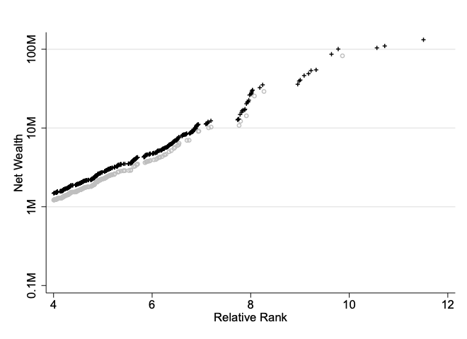
The following figure is the Pareto QQ-plot of (non-normalized) household net wealth, with + signs indicating observations from the SOEP-P sample, where we have zoomed into the upper tail for better visual clarity and have shifted down vertically observations form the SOEP sample (gray circles). SOEP-P clearly clusters in the upper tail of the distribution and thickens the upper tail of the net wealth distribution as observed in the SOEP. Apart from infilling, the SOEP-P sample also appends an upper tail.
Top wealth
beyondpareto yields the following estimate:
| k | Ybase | Std. Error | 95 % Conf. Int. | |
|---|---|---|---|---|
| 3,370 | 402,200 | 0.601 | 0.012 | (0.578, 0.623) |
(This is Table 1: Top wealth in Germany in 2019, Panel C. Optimal wealth threshold selection in RTTT, and Table 7 in the Stata Journal paper.)
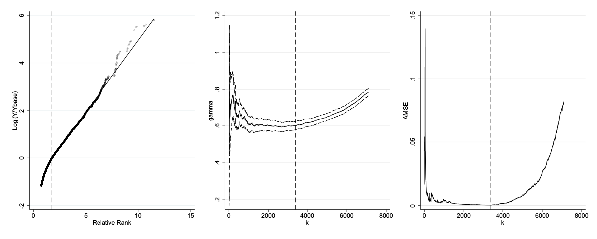
The next figure shows the full graphical output of
beyondpareto. At slightly more than 400,000 Euros, the
optimal threshold is lower than usual practitioners’ ad hoc threshold
choices (one or two million Euros in the German context). The associated
Pareto coefficient is a tightly estimated
,
indicating that wealth concentration in Germany is high. The Pareto-QQ
plot indicates that the Pareto distribution is a reasonable
approximation of household net wealth in Germany. The
and AMSE plots show that the selected thresholds imply an estimate of
from a stable and flat region.
Using this tail index estimate, applying
beyondpareto_topshares then yields the following estimates
of the top wealth concentration in Germany in 2019.
| Top 10% | Top 1% | |
|---|---|---|
| 0.601 | 57.45% | 22.90% |
The RTTT Replication Kit gives more details.
Wealth and income concentrations
SOEP-P is a fully integrated SOEP subsample, which means that all
variables are fully comparable across SOEP and SOEP-P, leading us to use
the shorthand SOEP+P for the combined data. We then
apply beyondpareto to various income concepts and obtain,
for instance, for market income a extreme value index estimate of 0.36,
and income shares for the top10 % earners of 31.53% and 7.24% for the
top earners.
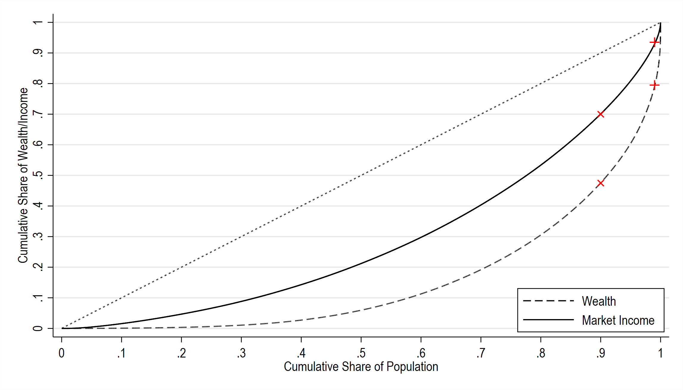
More generally, the next figure depicts the Lorenz curve (i.e. the plot of the cumulative income or wealth share against the cumulative population share) for both wealth and market income (the red crosses corresponding to the reported figures for the top 1% and 10%). It is evident that wealth in Germany is considerably more concentrated than income.
The key predictors of top wealth
In RTTT, we then proceed to identify the key predictors for belonging to the top 1 percent of income, wealth, and both distributions jointly. Although we consider many, only a few traits matter: Entrepreneurship and self-employment in conjunction with a sizable inheritance of company assets is the most important covariate combination across all rich groups. Our data suggest that all top 1 percent groups, but especially the joint top 1 percent, are predominantly populated by intergenerational entrepreneurs.
Top earnings and censored administrative data (based on SOEP-RV)
The following example is taken from
- “Dealing with Censored Earnings in Register Data”, Jahrbücher für Nationalökonomie und Statistik, 2025 (M. Beckmannshagen, J. König, I. Retter, C. Schluter, C. Schröder, Y. Tchokni). JBNST
Earnings are often top-coded (right-censored) in administrative registers. The censoring threshold in the case of Germany is the limit value for social security contributions, leading to a substantial fraction of censoring: For example, about 12% of male workers in West Germany are affected, rising to above 30% for highly educated prime-aged workers. This missing right tail of the earnings distribution constitutes a major problem for researchers studying earnings inequality and top incomes. We overcome this challenge by taking a distributional approach and semi-parametrically modelling the right tail as being Pareto-like. Non-censored earnings survey data matched to administrative records, derived from the SOEP-RV project, let us operate in a laboratory-like setting in which the targets are known.
SOEP-RV relies on a record linkage project with the German Pension Insurance. In this project, the survey data of the SOEP respondents have been linked 1:1 with their individual social security biography. We consider the sample of male workers in West Germany in 2019, the censoring incidence among West German men being 12.5%. We will use interchangeably “administrative earnings” and “Insurance Accounts (IA) earnings.”
In other words, we use beyond_pareto to estimate tail
index on the uncensored SOEP survey earnings data (which we label the
“target”), and the censored administrative (record-linked) earnings data
(IA earnings SOEP-RV), and compare the two.
We get the following estimates of and the top 1%, 5% and 10% earnings shares for male workers in West Germany in 2019 (the numbers are taken from Table 5: Tail estimation in the SOEP-RV sample of the paper):
| Ybase | 1% | 5% | 10% | ||
|---|---|---|---|---|---|
| Target (unrestricted, SOEP earn.) | 7,042 | 0.27 | 4.28 | 13.80 | 23.37 |
| Censored (IA earn.) | 6,266 | 0.24 | 3.81 | 12.86 | 21.72 |
The table reveals that our estimation approach gets close to the target value of = 0.27! Thus, we conclude that our estimation approach enables us to provide a credible estimate for the right tail of the earnings distribution based censored administrative earnings.
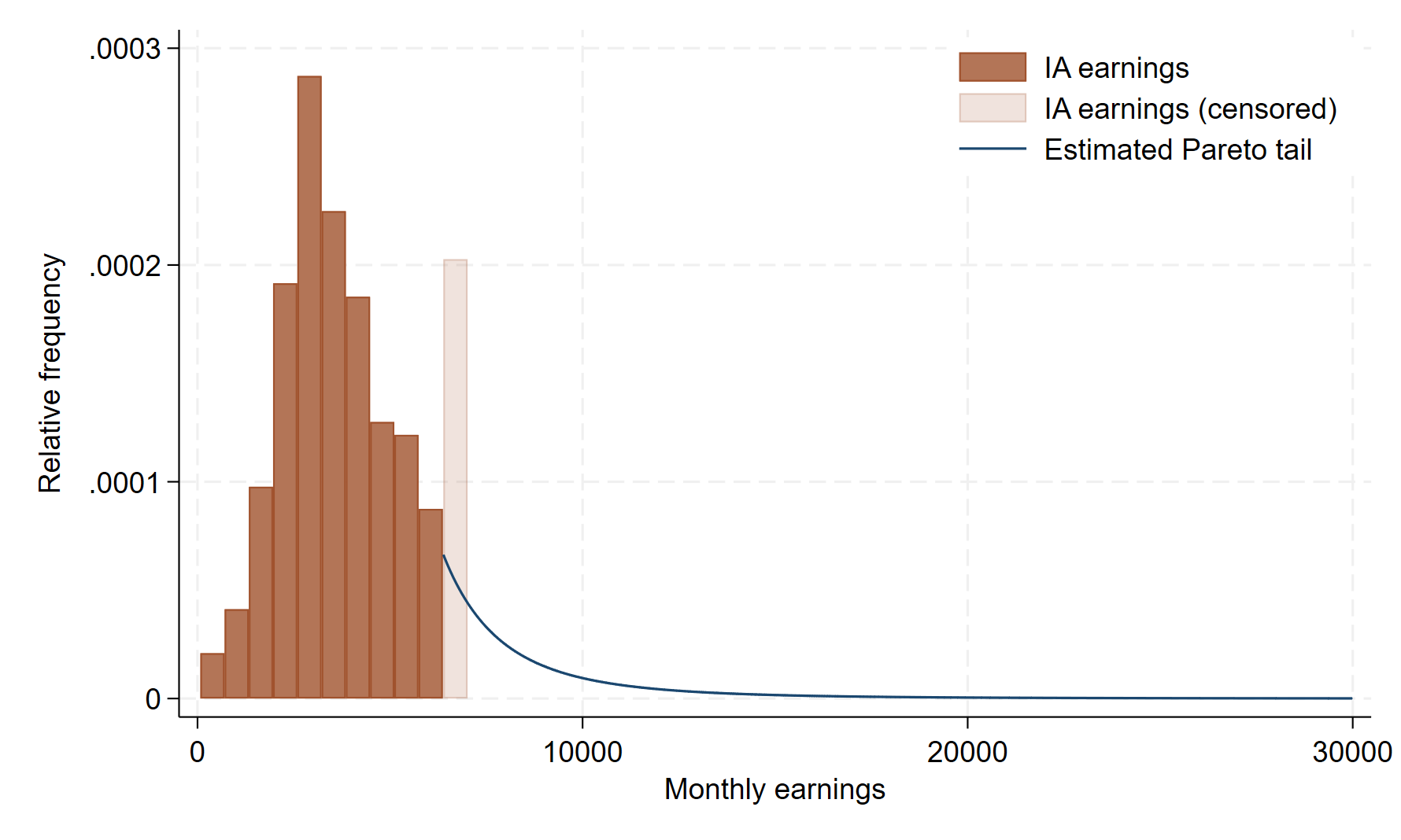
We visualizes the setting and the results: The histogram (brown bars) depicts the earnings density below the administrative censoring ceiling, as well as the mass point of the latter (transparent brown bar). We then smoothly paste a Pareto tail (blue line) based on our estimate .
Finally, we compare our earnings’ tail imputation to the target EDF (the uncensored survey data), and the EDF for a current-practice Tobit imputation.
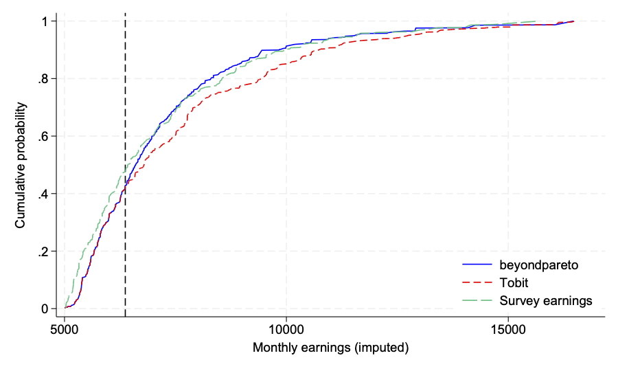
While the Tobit imputation does produce an approximation to the missing right tail of the censored earnings distribution that captures its heaviness fairly well, our CDF is always closer to the target EDF. The Tobit imputation systematically assigns earnings that are too large.