authored by Mattis Beckmannshagen, Johannes König, Isabella Retter, Christian Schluter, Carsten Schröder, Yogam Tchokni, published in Journal of Economics and Statistics, 2025. https://doi.org/10.1515/jbnst-2024-0037
The core functionality of the beyondpareto command used
for imputation of the censored right tail is described in the paper
König, Schluter, Schröder, Retter, and Beckmannshagen (2025),
“The beyondpareto command for optimal extreme value index
estimation,” The Stata Journal, 25(1) May 2025.
SJ
2025.
Installation: The package can be downloaded from The Stata Journal as
per usual, net sj 25-1.
Typing which beyondpareto yields
*! beyondpareto.ado, version 1.0, 2024-06-14
*! Christian Schluter and Isabella Retter
*! To learn more about beyondpareto see the vignette at
*! https://christianschluter.github.io/beyondpareto/The data set used here is the German Socio-Economic Panel. We are not allowed to share the data. However, it is available, free of charge, to researchers worldwide, upon entering into a data contract, see details. The full replication code (data generation, all computations) is deposited in the Reanalysis archive of the SOEP Research Data Center (SOEP-RDC).
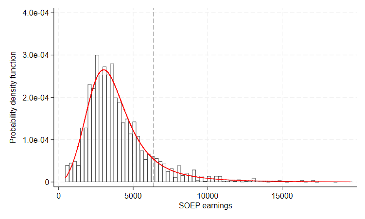
We illustrate the main procedure (and a proof of concept and performance evidence) using artificial data. So that the model be realistic, we fit the parametric model to monthly earnings data taken from the SOEP for male workers in West Germany in 2018, stored in the variable inc_soep. Specifically, we fit the data using a highly flexible distribution, the generalized beta distribution of the second kind (GB2), with the density function \[ GB2(y;a,b,p,q)={\frac {|a|y^{ap-1}}{b^{ap}B(p,q)(1+(y/b)^{a})^{p+q}}}, \quad \quad \quad (y,a,b,p,q >0).\]
. gb2fit inc_soep , svy stats from(4 3500 0.7 0.8, copy) pdf(pdfgb2) poorfrac(6370)

Initial:      Log pseudolikelihood = -1.068e+08
Rescale:      Log pseudolikelihood = -1.068e+08
Rescale eq:   Log pseudolikelihood = -1.068e+08
Iteration 0:  Log pseudolikelihood = -1.068e+08
Iteration 1:  Log pseudolikelihood = -1.067e+08
Iteration 2:  Log pseudolikelihood = -1.067e+08
Iteration 3:  Log pseudolikelihood = -1.067e+08
Iteration 4:  Log pseudolikelihood = -1.067e+08
Iteration 5:  Log pseudolikelihood = -1.067e+08

ML fit of GB2 distribution

pweight:  phrf                                    Number of obs    =      4444
Strata:   <one>                                   Number of strata =         1
PSU:      <observations>                          Number of PSUs   =      4444
                                                  Population size  =  11939209
                                                  F(   0,   4444)  =         .
                                                  Prob > F         =         .

─────────────┬────────────────────────────────────────────────────────────────
    inc_soep │ Coefficient  Std. err.      t    P>|t|     [95% conf. interval]
─────────────┼────────────────────────────────────────────────────────────────
a            │
       _cons │   4.037141   .6002606     6.73   0.000     2.860331     5.21395
─────────────┼────────────────────────────────────────────────────────────────
b            │
       _cons │   3633.295   135.1821    26.88   0.000     3368.271    3898.319
─────────────┼────────────────────────────────────────────────────────────────
p            │
       _cons │   .7572215   .1397604     5.42   0.000     .4832216    1.031222
─────────────┼────────────────────────────────────────────────────────────────
q            │
       _cons │   .8250917   .1767598     4.67   0.000     .4785543    1.171629
─────────────┴────────────────────────────────────────────────────────────────

Fraction with  inc_soep < 6370 =   0.88780

────────────────────────────────────────────────────────────
     Quantiles       Cumulative shares of
                     total inc_soep (Lorenz ordinates)
────────────────────────────────────────────────────────────
 1%  849.49997       0.00158
 5%   1.44e+03       0.01343
10%   1.83e+03       0.03382
20%   2.34e+03       0.08576
25%   2.55e+03       0.11605
30%   2.75e+03       0.14885
40%   3.13e+03       0.22158 Mode         3.02e+03
50%   3.52e+03       0.30374 Mean         4.04e+03
60%   3.95e+03       0.39598 Std. Dev.    2.66e+03
70%   4.48e+03       0.50000
75%   4.82e+03       0.55744 Variance     7.08e+06
80%   5.23e+03       0.61945 Half CV^2     0.21646
90%   6.61e+03       0.76357
95%   8.23e+03       0.85389 p90/p10       3.61841
99%   1.34e+04       0.95251 p75/p25       1.88657
────────────────────────────────────────────────────────────

.
. twoway  (hist inc_soep [fw=int(phrf)] if inc_soep<20000, width(250) lcol(black) fcol(none)) (connected  pdfgb2 inc_soe
> p if inc_soep<20000, msize(vtiny) mc(red) lc(red) msymbol(circle_hollow)), xline(6370, lc(gs10) lp(dash)) legend(off)
> xtitle(SOEP earnings) ytitle(Probability density function) name(male, replace) xscale(range(0 17500)) xlabel(0 (5000)
> 15000) yscale(range(0 0.0004)) ylabel(0 (.0001) .0004)
We then use the fitted GB2 model as our data generating process (DGP), with true tail parameter \(\gamma = .304\) and an implied true earnings share for the top 1% of 4.8%.
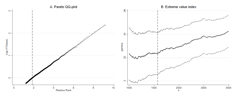
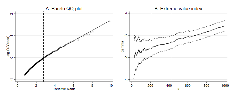
Figure 2 illustrates the estimator of \(\gamma\) for one such random sample using
beyondpareto. Panel (A) depicts the Pareto QQ-plot for the
upper earnings tail and shows its approximate linearity. We fit a
straight line with slope \(\widehat{\gamma}\); the vertical dashed
line depicts the value corresponding to the optimally determined \(Y_{base}\). In panel (B), we depict \(\widehat{\gamma}\) as a function of the
upper order statistics \(k\), and the
optimal \(k^*\) corresponds to \(Y_{base}\). Beyond this \(k^*\), the estimator is increasingly
distorted.
. clear

. set seed 330033

. local a = 3633.295

. local b = 4.037

. local p = 0.757

. local q = 0.825

. qui set obs 10000

. qui gen double income =  `a'*( (1/invibeta(`p',`q',runiform()))-1  )^(-1/`b')

. beyondpareto income, plot(pareto) nrange(1000,3000)
No sampling weights given. Using w=1.
Considering the top 3000 of 10000 values, starting from the first 1000 and testing 2001 values for k base.

──────────┬───────────────────────────────────────────────────────────
  Results │      Ybase       gamma        S.E.  [95% Conf.   Interval]
──────────┼───────────────────────────────────────────────────────────
   income │  5810.3139   .32328834    .0091105    .3054318    .3411449
──────────┴───────────────────────────────────────────────────────────
Optimal k base: 1574

. gr_edit title.text.Arrpush A: Pareto QQ-plot

. qui beyondpareto income, plot(gamma) nrange(1000,3000)

. gr_edit title.text.Arrpush B: Extreme value index

. graph combine QQ gamma

. graph display, xsize(12) ysize(5)

. graph export gb2_plots.png, replace
file gb2_plots.png saved as PNG format
Is the good fit for this one synthetic distribution just a coincidence? To answer this question, we perform a Monte Carlo study, generating 1,000 synthetic distributions of size 10,000. For each synthetic distribution, we estimate the extreme value index γ. For this task, the values for the parameters a,b,p,q that were estimated above,
\(a = 4.037,\ b =3633.295, \ p =0.757, \ q =0.825,\)
have to be inserted into beyondpareto_GB2sim.ado which is distributed with this replication code.
Bottom line: In this lab setting, beyondpareto performs
very well: the estimated values are very close to the true population
values and the empirical standard deviations across simulations suggest
tight estimates.
Figure 3 is a scatter plot to show that insurance accounts (IA) earnings and self-reported SOEP earnings are highly correlated. If high correlation below the censoring threshold is given, we can use survey earnings as a good benchmark also for (imputed) earnings above the censoring threshold. As an example, we plot the earnings in the year 2018 for record- linked men in West Germany with IA earnings below the assessment ceiling of €6,370. The black line is the 45-degree bisector, the red functional form shows the result of a locally weighted regression—and thus a highly flexible form. The figure shows that both earnings variables are highly correlated with a correlation coefficient \(\rho\) of 0.92.
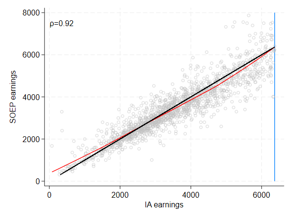
Bottom line: The two earnings concepts are highly correlated. SOEP-RV can thus be considered an ideal laboratory to assess the performance of imputation methods.
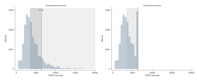
Our benchmarking of the beyondpareto approach relies on
a comparison of three scenarios, illustrated in Figure 4:
The left-hand panel of Figure 4 shows the distribution of uncensored
SOEP earnings. In scenario 1, the target scenario,
beyondpareto determines the optimal \(Y_{base}\) within the whole range depicted
by the shaded areas A and B. In the restricted scenario,
beyondpareto will only consider area A, below the censoring
threshold. The right-hand panel show the artificially censored SOEP
earnings, including the mass point at the censoring threshold. The area
under consideration for beyondpareto in the censored
setting is again displayed by the shaded area.
We now apply beyondpareto in the three described
scenarios for the case of 2018, based on the full SOEP sample. In the
paper, we also consider the years 2014-2017 and 2019.
. use ${temp}soep_west.dta, clear
(SOEP-Core, v38.1 (EU Edition), doi:10.5684/soep.core.v38.1eu)

. keep if JAHR ==2018 & syear==2018 // only use 2018
(57,313 observations deleted)

. keep if sex==1 // focus on men
(4,227 observations deleted)

. gen weight= phrf

. sum BMG_WEST if syear ==2018

    Variable │        Obs        Mean    Std. dev.       Min        Max
─────────────┼─────────────────────────────────────────────────────────
    BMG_WEST │      4,444        6500           0       6500       6500

. global sc_limit=r(mean)

. global lm = 0.98 * $sc_limit

. mat out=J(5,6,.)

. **************************************************
. *(a) target/unrestricted
. **************************************************
. preserve

. collapse (sum) weight, by(inc_soep)

. *beyondpareto inc_soep [w=weight] , nrange(20, 1000)
. *diagnose plot (here figure 5 is produced)
. beyondpareto inc_soep [w=weight] , nrange(20, 1000) plot(pareto) save(${out}4a_pareto.png, width(1200) replace)
(sampling weights assumed)
Using the given sampling weights.
Considering the top 1000 of 1851 values, starting from the first 20 and testing 981 values for k base.

──────────┬───────────────────────────────────────────────────────────
  Results │      Ybase       gamma        S.E.  [95% Conf.   Interval]
──────────┼───────────────────────────────────────────────────────────
 inc_soep │  7991.6665   .23670794    .0183943    .2006552    .2727607
──────────┴───────────────────────────────────────────────────────────
Optimal k base: 207
Saving plots

. gr_edit title.text.Arrpush A: Pareto QQ-plot

. beyondpareto inc_soep [w=weight] , nrange(20, 1000) plot(gamma) save(${out}4a_gamma.png, width(1200) replace)
(sampling weights assumed)
Using the given sampling weights.
Considering the top 1000 of 1851 values, starting from the first 20 and testing 981 values for k base.

──────────┬───────────────────────────────────────────────────────────
  Results │      Ybase       gamma        S.E.  [95% Conf.   Interval]
──────────┼───────────────────────────────────────────────────────────
 inc_soep │  7991.6665   .23670794    .0183943    .2006552    .2727607
──────────┴───────────────────────────────────────────────────────────
Optimal k base: 207
Saving plots

. gr_edit title.text.Arrpush B: Extreme value index

. addplot: , xline(430, lp(tight_dot) lc(black))

. graph combine QQ gamma, iscale(1)

. graph display, xsize(12) ysize(5)

. graph export 4a_pareto_gamma_comb.png, replace
file 4a_pareto_gamma_comb.png saved as PNG format

. mat out[2,1] =  e(Ybase)

. mat out[2,2] = e(gamma)

. // sum of all weights, of weighted tail, and of all censored individuals
. sum weight if inc_soep >e(Ybase)

    Variable │        Obs        Mean    Std. dev.       Min        Max
─────────────┼─────────────────────────────────────────────────────────
      weight │        206    3616.483    5894.219      37.17   56524.53

. scalar w_flanke=r(sum)

. sum weight if inc_soep >=$lm

    Variable │        Obs        Mean    Std. dev.       Min        Max
─────────────┼─────────────────────────────────────────────────────────
      weight │        370    3935.221    5667.319      37.17   56524.53

. scalar w_cens=r(sum)

. sum weight if !missing(inc_soep)

    Variable │        Obs        Mean    Std. dev.       Min        Max
─────────────┼─────────────────────────────────────────────────────────
      weight │      1,851     6450.14    14708.13       13.5   220120.6

. scalar w_all=r(sum)

. scalar rel_k_opt=w_flanke/w_all -0.0000001

. scalar rel_cens=w_cens/w_all

. // store shares
. beyondpareto_topshares inc_soep [w=weight], shares(0.01 0.05 0.1) matname(topshares)
(sampling weights assumed)
Using the following results for gamma: .23670794 and Ybase: 7991.6665
Using the given sampling weights.

. mat out[2,3] = e(topshares)[1,2]

. mat out[2,4] = e(topshares)[2,2]

. // Top 10 percent also include individuals outside of the tail. Therefore we have to calculate the earnings share of t
> he tail (based on beyondpareto_topshares) and of the individuals between the 90th percentile and the beginning of the
> tail
. *compute share of tail (excluding ybase)
. beyondpareto_topshares inc_soep [w=weight], shares(`=rel_k_opt') matname("tail")
(sampling weights assumed)
Using the following results for gamma: .23670794 and Ybase: 7991.6665
Using the given sampling weights.

. * compute share between BBG/p90 and tail
. sum inc_soep [w=weight],d
(analytic weights assumed)

                          inc_soep
─────────────────────────────────────────────────────────────
      Percentiles      Smallest
 1%     708.3333       454.1667
 5%         1500            460
10%         1900          462.5       Obs               1,851
25%     2516.667       462.5833       Sum of wgt.  11939208.7

50%         3500                      Mean           4021.874
                        Largest       Std. dev.      2337.413
75%     4895.833       23133.33
90%     6733.333       24916.67       Variance        5463498
95%         8350       25833.33       Skewness        2.43301
99%     12866.67          41000       Kurtosis        15.6383

. scalar inc_total = r(sum)

. scalar p90=r(p90)

. sum inc_soep if inc_soep>=$lm & inc_soep<=e(Ybase) [w=weight]
(analytic weights assumed)

    Variable │     Obs      Weight        Mean   Std. dev.       Min        Max
─────────────┼─────────────────────────────────────────────────────────────────
    inc_soep │     164  711036.419    6981.765   418.4139       6375   7991.667

. scalar share_lm_bbg = r(sum)/inc_total

. sum inc_soep if inc_soep>=p90 & inc_soep<=e(Ybase) [w=weight]
(analytic weights assumed)

    Variable │     Obs      Weight        Mean   Std. dev.       Min        Max
─────────────┼─────────────────────────────────────────────────────────────────
    inc_soep │     118  458627.469    7216.794   330.2441   6733.333   7991.667

. scalar share_p90_ybase=r(sum)/inc_total

. * add up share of tail with the respective share below
. mat out[2,5] =  e(tail)[1,2] + 100*share_p90_ybase

. mat out[2,6] = e(tail)[1,2] + 100*share_lm_bbg

. restore

. **************************************************
. *(b) restricted, Ybase forced to be below BBG by setting k min left
. **************************************************
. preserve

. collapse (sum) weight, by(inc_soep)

. sum inc_soep if inc_soep>0.98*$sc_limit

    Variable │        Obs        Mean    Std. dev.       Min        Max
─────────────┼─────────────────────────────────────────────────────────
    inc_soep │        370    9480.188    3787.074       6375      41000

. local n_cens_soep=r(N)

. sum inc_soep

    Variable │        Obs        Mean    Std. dev.       Min        Max
─────────────┼─────────────────────────────────────────────────────────
    inc_soep │      1,851    4597.373    3240.883   454.1667      41000

. local n_total = r(N)

. local min_b = `n_cens_soep' + 20

. beyondpareto inc_soep [w=weight] , nrange(`min_b', 1000)
(sampling weights assumed)
Using the given sampling weights.
Considering the top 1000 of 1851 values, starting from the first 390 and testing 611 values for k base.

──────────┬───────────────────────────────────────────────────────────
  Results │      Ybase       gamma        S.E.  [95% Conf.   Interval]
──────────┼───────────────────────────────────────────────────────────
 inc_soep │       6200   .26419235    .0148059    .2351729    .2932118
──────────┴───────────────────────────────────────────────────────────
Optimal k base: 398

. mat out[3,1] = e(Ybase)

. mat out[3,2] = e(gamma)

. // store shares
. beyondpareto_topshares inc_soep [w=weight], shares(0.01, 0.05, 0.10) matname("topshares")
(sampling weights assumed)
Using the following results for gamma: .26419235 and Ybase: 6200
Using the given sampling weights.

. mat out[3,3] = e(topshares)[1,2]

. mat out[3,4] = e(topshares)[2,2]

. mat out[3,5] = e(topshares)[3,2]

. sum weight if inc_soep >=$lm

    Variable │        Obs        Mean    Std. dev.       Min        Max
─────────────┼─────────────────────────────────────────────────────────
      weight │        370    3935.221    5667.319      37.17   56524.53

. scalar w_cens=r(sum)

. sum weight if !missing(inc_soep)

    Variable │        Obs        Mean    Std. dev.       Min        Max
─────────────┼─────────────────────────────────────────────────────────
      weight │      1,851     6450.14    14708.13       13.5   220120.6

. scalar w_all=r(sum)

. scalar rel_cens=w_cens/w_all

. *compute share of censored
. beyondpareto_topshares inc_soep [w=weight], shares(`=rel_cens') matname("censored")
(sampling weights assumed)
Using the following results for gamma: .26419235 and Ybase: 6200
Using the given sampling weights.

. mat out[3,6] = e(censored)[1,2]

. restore

. **************************************************
. *(c) (artificially) censored
. **************************************************
. preserve

. collapse (sum) weight, by(inc_soep)

. * artificial censoring and correction of mass point (adding the weight of the censored to the last uncensored obs.)
. sum weight if inc_soep>=$lm

    Variable │        Obs        Mean    Std. dev.       Min        Max
─────────────┼─────────────────────────────────────────────────────────
      weight │        370    3935.221    5667.319      37.17   56524.53

. local sumwcens = r(sum)

. sum inc_soep if inc_soep<$lm

    Variable │        Obs        Mean    Std. dev.       Min        Max
─────────────┼─────────────────────────────────────────────────────────
    inc_soep │      1,481    3377.494    1450.441   454.1667   6366.667

. replace weight = weight + `sumwcens' if inc_soep==r(max)
(1 real change made)

. replace inc_soep=. if inc_soep>=$lm
(370 real changes made, 370 to missing)

. beyondpareto inc_soep [w=weight] , nrange(20, 1000)
(sampling weights assumed)
(370 missing values generated)
Using the given sampling weights.
Considering the top 1000 of 1481 values, starting from the first 20 and testing 981 values for k base.

──────────┬───────────────────────────────────────────────────────────
  Results │      Ybase       gamma        S.E.  [95% Conf.   Interval]
──────────┼───────────────────────────────────────────────────────────
 inc_soep │  6239.1665   .26662029    .0621562    .1447942    .3884464
──────────┴───────────────────────────────────────────────────────────
Optimal k base: 23

. mat out[4,1] = e(Ybase)

. mat out[4,2] = e(gamma)

. beyondpareto_topshares inc_soep [w=weight], shares(0.01, 0.05, 0.10) matname("shares")
(sampling weights assumed)
Using the following results for gamma: .26662029 and Ybase: 6239.1665
(370 missing values generated)
Using the given sampling weights.

. // store shares
. mat out[4,3] = e(shares)[1,2]

. mat out[4,4] = e(shares)[2,2]

. mat out[4,5] = e(shares)[3,2]

. sum weight if inc_soep >=$lm

    Variable │        Obs        Mean    Std. dev.       Min        Max
─────────────┼─────────────────────────────────────────────────────────
      weight │        370    3935.221    5667.319      37.17   56524.53

. scalar w_cens=r(sum)

. sum weight if !missing(inc_soep)

    Variable │        Obs        Mean    Std. dev.       Min        Max
─────────────┼─────────────────────────────────────────────────────────
      weight │      1,481    8061.586    41008.82       13.5    1457932

. scalar w_all=r(sum)

. scalar rel_k_opt=w_flanke/w_all

. scalar rel_cens=w_cens/w_all

. *compute share of censored
. beyondpareto_topshares inc_soep [w=weight], shares(`=rel_cens') matname("censored")
(sampling weights assumed)
Using the following results for gamma: .26662029 and Ybase: 6239.1665
(370 missing values generated)
Using the given sampling weights.

. mat out[4,6] = e(censored)[1,2]

. mat out2=out[2..4,1..6]

. restore

. frmttable using table3.tex, statmat(out2) multicol(1,2,2;1,4,4) rtitle("Target (unrestricted)" \ "Restricted"\"Censore
> d") ctitle("", "Tail metrics" , "" , "Top earnings shares", "", "", "" \"", " $ Y_{base}$", " $\hat{\gamma} $" ,"1\%",
> "5\%","10\%", "Cens.\%") tex fr replace sdec(0,2,2,2,2,2)

         ─────────────────────────────────────────────────────────────────────────────────────────────────────
                                  Tail metrics                    Top earnings shares
                                   $ Y_{base}$   $\hat{\gamma} $          1\%           5\%   10\%   Cens.\%
         ─────────────────────────────────────────────────────────────────────────────────────────────────────
          Target (unrestricted)      7,992            0.24               4.01          13.71  23.13   26.57
          Restricted                 6,200            0.26               4.16          13.59  22.63   26.19
          Censored                   6,239            0.27               4.21          13.70  22.78   26.35
         ─────────────────────────────────────────────────────────────────────────────────────────────────────
Figure 5 shows the diagnostic plots of beyondpareto for
the target scenario in the SOEP sample. The dotted line (Panel B)
represents the optimal Y_base in the restricted setting.
Bottom line: From Table 3, we conclude that censoring of the data at the assessment ceiling does not prevent us from achieving a very good approximation of the tail of the earnings distribution.
We now consider the smaller SOEP-RV sample and report the results in Table 5.
. use ${temp}soep_rv_west.dta, clear
(SOEP-Core, v38.1 (EU Edition), doi:10.5684/soep.core.v38.1eu)

. keep if JAHR ==2018 // only use 2018
(0 observations deleted)

. keep if sex==1 // focus on men
(1,997 observations deleted)

. gen weight= phrf

. *Output matrix
. mat out2=J(6,6,.)

. sum BMG_WEST if syear ==2018

    Variable │        Obs        Mean    Std. dev.       Min        Max
─────────────┼─────────────────────────────────────────────────────────
    BMG_WEST │      1,920        6500           0       6500       6500

. global sc_limit=r(mean)

. global lm = 0.98 * $sc_limit

. **************************************************
. *(a) unrestricted (target)
. **************************************************
. preserve

. collapse (sum) weight, by(inc_soep)

. beyondpareto inc_soep [w=weight] , nrange(20, 1000)
(sampling weights assumed)
Using the given sampling weights.
Considering the top 1000 of 1110 values, starting from the first 20 and testing 981 values for k base.

──────────┬───────────────────────────────────────────────────────────
  Results │      Ybase       gamma        S.E.  [95% Conf.   Interval]
──────────┼───────────────────────────────────────────────────────────
 inc_soep │       6200   .27431101    .0198381    .2354284    .3131936
──────────┴───────────────────────────────────────────────────────────
Optimal k base: 239

. mat out2[2,1] = e(Ybase)

. mat out2[2,2] = e(gamma)

. sum weight if inc_soep >=$lm

    Variable │        Obs        Mean    Std. dev.       Min        Max
─────────────┼─────────────────────────────────────────────────────────
      weight │        221    3094.013    3852.989      37.17   24529.21

. scalar w_cens=r(sum)

. sum weight if !missing(inc_soep)

    Variable │        Obs        Mean    Std. dev.       Min        Max
─────────────┼─────────────────────────────────────────────────────────
      weight │      1,115    5086.979    8481.022          0   103471.4

. scalar w_all=r(sum)

. scalar rel_cens=w_cens/w_all

. // store shares
. beyondpareto_topshares inc_soep [w=weight], shares(0.01 0.05 0.1) matname(topshares)
(sampling weights assumed)
Using the following results for gamma: .27431101 and Ybase: 6200
Using the given sampling weights.

. mat out2[2,3] = e(topshares)[1,2]

. mat out2[2,4] = e(topshares)[2,2]

. mat out2[2,5] = e(topshares)[3,2]

. *compute share of censored (which are all part of the tail)
. beyondpareto_topshares inc_soep [w=weight], shares(`=rel_cens-0.00001') matname("cens")
(sampling weights assumed)
Using the following results for gamma: .27431101 and Ybase: 6200
Using the given sampling weights.

. mat out2[2,6] = e(cens)[1,2]

. restore

. **************************************************
. *(b) restricted, Ybase forced to be below BBG
. **************************************************
. preserve

. collapse (sum) weight, by(inc_soep)

. sum inc_soep if inc_soep>=0.98*$sc_limit

    Variable │        Obs        Mean    Std. dev.       Min        Max
─────────────┼─────────────────────────────────────────────────────────
    inc_soep │        221     9149.34    3785.501       6375      41000

. local n_cens_soep=r(N)

. sum inc_soep

    Variable │        Obs        Mean    Std. dev.       Min        Max
─────────────┼─────────────────────────────────────────────────────────
    inc_soep │      1,115    4603.961    3076.559        310      41000

. local n_total = r(N)

. local min_b = `n_cens_soep' + 20

. beyondpareto inc_soep [w=weight] , nrange(`n_cens_soep', 400)
(sampling weights assumed)
Using the given sampling weights.
Considering the top 400 of 1110 values, starting from the first 221 and testing 180 values for k base.

──────────┬───────────────────────────────────────────────────────────
  Results │      Ybase       gamma        S.E.  [95% Conf.   Interval]
──────────┼───────────────────────────────────────────────────────────
 inc_soep │       6200   .27431101    .0198381    .2354284    .3131936
──────────┴───────────────────────────────────────────────────────────
Optimal k base: 239

. mat out2[3,1] = e(Ybase)

. mat out2[3,2] = e(gamma)

. // store shares
. beyondpareto_topshares inc_soep [w=weight], shares(0.01, 0.05, 0.10) matname("topshares")
(sampling weights assumed)
Using the following results for gamma: .27431101 and Ybase: 6200
Using the given sampling weights.

. mat out2[3,3] = e(topshares)[1,2]

. mat out2[3,4] = e(topshares)[2,2]

. mat out2[3,5] = e(topshares)[3,2]

. sum weight if inc_soep >=$lm

    Variable │        Obs        Mean    Std. dev.       Min        Max
─────────────┼─────────────────────────────────────────────────────────
      weight │        221    3094.013    3852.989      37.17   24529.21

. scalar w_cens=r(sum)

. sum weight if !missing(inc_soep)

    Variable │        Obs        Mean    Std. dev.       Min        Max
─────────────┼─────────────────────────────────────────────────────────
      weight │      1,115    5086.979    8481.022          0   103471.4

. scalar w_all=r(sum)

. scalar rel_cens=w_cens/w_all

. *compute share of censored (which are all part of the tail)
. beyondpareto_topshares inc_soep [w=weight], shares(`=rel_cens-0.00001') matname("cens")
(sampling weights assumed)
Using the following results for gamma: .27431101 and Ybase: 6200
Using the given sampling weights.

. mat out2[3,6] = e(cens)[1,2]

. restore

. **************************************************
. *(c) censored (artifically) SOEP earnings
. **************************************************
. preserve

. collapse (sum) weight, by(inc_soep)

. * artificial censoring and correction of mass point (adding the weight of the censored to the last uncensored obs.)
. sum weight if inc_soep>=$lm

    Variable │        Obs        Mean    Std. dev.       Min        Max
─────────────┼─────────────────────────────────────────────────────────
      weight │        221    3094.013    3852.989      37.17   24529.21

. local sumwcens = r(sum)

. sum inc_soep if inc_soep<$lm

    Variable │        Obs        Mean    Std. dev.       Min        Max
─────────────┼─────────────────────────────────────────────────────────
    inc_soep │        894    3480.327     1378.51        310   6366.667

. replace weight = weight + `sumwcens' if inc_soep==r(max)
(1 real change made)

. replace inc_soep=. if inc_soep>=$lm
(221 real changes made, 221 to missing)

. beyondpareto inc_soep [w=weight] , nrange(15, 500)
(sampling weights assumed)
(221 missing values generated)
Using the given sampling weights.
Considering the top 500 of 889 values, starting from the first 15 and testing 486 values for k base.

──────────┬───────────────────────────────────────────────────────────
  Results │      Ybase       gamma        S.E.  [95% Conf.   Interval]
──────────┼───────────────────────────────────────────────────────────
 inc_soep │       6200   .26233101    .0691303    .1268356    .3978264
──────────┴───────────────────────────────────────────────────────────
Optimal k base: 18

. mat out2[4,1] = e(Ybase)

. mat out2[4,2] = e(gamma)

. beyondpareto_topshares inc_soep [w=weight], shares(0.01, 0.05, 0.10) matname("shares")
(sampling weights assumed)
Using the following results for gamma: .26233101 and Ybase: 6200
(221 missing values generated)
Using the given sampling weights.

. // store shares
. mat out2[4,3] = e(shares)[1,2]

. mat out2[4,4] = e(shares)[2,2]

. mat out2[4,5] = e(shares)[3,2]

. sum weight if inc_soep >=$lm

    Variable │        Obs        Mean    Std. dev.       Min        Max
─────────────┼─────────────────────────────────────────────────────────
      weight │        221    3094.013    3852.989      37.17   24529.21

. scalar w_cens=r(sum)

. sum weight if !missing(inc_soep)

    Variable │        Obs        Mean    Std. dev.       Min        Max
─────────────┼─────────────────────────────────────────────────────────
      weight │        894    6344.498    24539.72          0     685677

. scalar w_all=r(sum)

. scalar rel_cens=w_cens/w_all

. *compute share of censored
. beyondpareto_topshares inc_soep [w=weight], shares(`=rel_cens') matname("cens")
(sampling weights assumed)
Using the following results for gamma: .26233101 and Ybase: 6200
(221 missing values generated)
Using the given sampling weights.

. mat out2[4,6] = e(cens)[1,2]

. restore

. **************************************************
.  *(d) censored ⇒ IA earnings
. **************************************************
. preserve

. collapse (sum) weight, by(inc_vskt_cens)

. * artificial censoring and correction of mass point (adding the weight of the censored to the last uncensored obs.)
. sum weight if inc_vskt_cens>=$lm

    Variable │        Obs        Mean    Std. dev.       Min        Max
─────────────┼─────────────────────────────────────────────────────────
      weight │          1    724466.9           .   724466.9   724466.9

. local sumwcens = r(sum)

. sum inc_vskt_cens if inc_vskt_cens<$lm

    Variable │        Obs        Mean    Std. dev.       Min        Max
─────────────┼─────────────────────────────────────────────────────────
inc_vskt_c~s │      1,509    3521.433    1364.214   73.58871   6367.876

. replace weight = weight + `sumwcens' if inc_vskt_cens==r(max)
(1 real change made)

. replace inc_vskt_cens=. if inc_vskt_cens>=$lm
(1 real change made, 1 to missing)

. beyondpareto inc_vskt_cens [w=weight] , nrange(20, 400)
(sampling weights assumed)
(1 missing value generated)
Using the given sampling weights.
Considering the top 400 of 1502 values, starting from the first 20 and testing 381 values for k base.

──────────────┬───────────────────────────────────────────────────────────
      Results │      Ybase       gamma        S.E.  [95% Conf.   Interval]
──────────────┼───────────────────────────────────────────────────────────
inc_vskt_cens │  6265.8335   .24398702    .0609968    .1244334    .3635406
──────────────┴───────────────────────────────────────────────────────────
Optimal k base: 20

. mat out2[5,1] = e(Ybase)

. mat out2[5,2] = e(gamma)

. beyondpareto_topshares inc_vskt_cens [w=weight], shares(0.01, 0.05, 0.10) matname("shares")
(sampling weights assumed)
Using the following results for gamma: .24398702 and Ybase: 6265.8335
(1 missing value generated)
Using the given sampling weights.

. // store shares
. mat out2[5,3] = e(shares)[1,2]

. mat out2[5,4] = e(shares)[2,2]

. mat out2[5,5] = e(shares)[3,2]

. sum weight if inc_vskt_cens >=$lm

    Variable │        Obs        Mean    Std. dev.       Min        Max
─────────────┼─────────────────────────────────────────────────────────
      weight │          1    724466.9           .   724466.9   724466.9

. scalar w_cens=r(sum)

. sum weight if !missing(inc_vskt_cens)

    Variable │        Obs        Mean    Std. dev.       Min        Max
─────────────┼─────────────────────────────────────────────────────────
      weight │      1,509    3758.768    19139.36          0   732632.7

. scalar w_all=r(sum)

. scalar rel_cens=w_cens/w_all

. *compute share of censored
. beyondpareto_topshares inc_vskt_cens [w=weight], shares(`=rel_cens') matname("cens")
(sampling weights assumed)
Using the following results for gamma: .24398702 and Ybase: 6265.8335
(1 missing value generated)
Using the given sampling weights.

. mat out2[5,6] = e(cens)[1,2]

. mat out2=out2[2..5,1..6]

. restore

. ***compute table***
. frmttable using table5.tex, statmat(out2) multicol(1,2,2;1,4,4) rtitle("Target (unrestricted, SOEP earn.)" \ "Restrict
> ed (SOEP earn.)"\"Censored (SOEP earn.)"\"Censored (IA earn.)") ctitle("", "Tail metrics" , "" , "Top earnings shares"
> , "", "", "" \"", " $ Y_{base}$", " $\hat{\gamma} $" ,"1\%","5\%","10\%", "Cens.\%") tex fr replace sdec(0,2,2,2,2,2)

   ─────────────────────────────────────────────────────────────────────────────────────────────────────────────────
                                        Tail metrics                    Top earnings shares
                                         $ Y_{base}$   $\hat{\gamma} $          1\%           5\%   10\%   Cens.\%
   ─────────────────────────────────────────────────────────────────────────────────────────────────────────────────
    Target (unrestricted, SOEP earn.)      6,200            0.27               4.27          13.74  22.73   26.03
    Restricted (SOEP earn.)                6,200            0.27               4.27          13.74  22.73   26.03
    Censored (SOEP earn.)                  6,200            0.26               4.10          13.43  22.39   25.70
    Censored (IA earn.)                    6,266            0.24               3.81          12.86  21.72   26.13
   ─────────────────────────────────────────────────────────────────────────────────────────────────────────────────
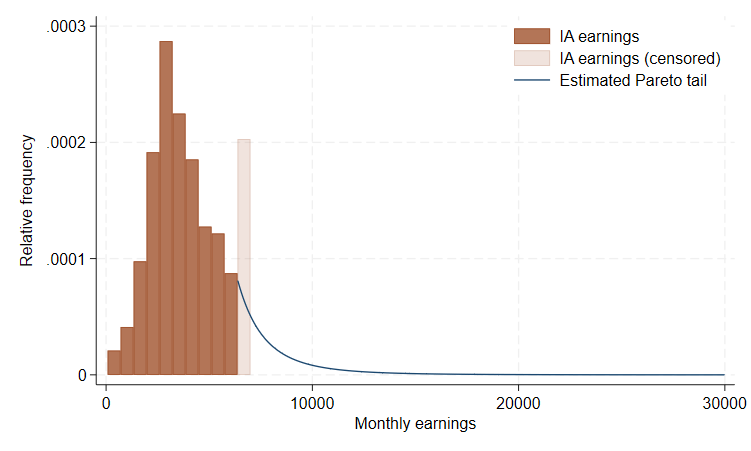
Bottom line: Our estimation approach enables us to provide a credible estimate for the right tail of the earnings distribution based on censored administrative earnings. Figure 6 visualizes the setting and the results: The histogram (brown bars) depicts the earnings density below the administrative censoring ceiling alongside the mass point of the latter (transparent brown bar). We then smoothly paste a Pareto tail (blue line) based on our estimate of \(\hat{\gamma}= 0.24\).
. use ${temp}soep_rv_west.dta, clear
(SOEP-Core, v38.1 (EU Edition), doi:10.5684/soep.core.v38.1eu)

. // only use 2018
. keep if JAHR ==2018
(0 observations deleted)

. keep if sex==1
(1,997 observations deleted)

. gen weight= phrf

. sum BMG_WEST if syear ==2018

    Variable │        Obs        Mean    Std. dev.       Min        Max
─────────────┼─────────────────────────────────────────────────────────
    BMG_WEST │      1,920        6500           0       6500       6500

. global sc_limit=r(mean)

. global lm = 0.98 * $sc_limit

. preserve

. keep inc_vskt_cens weight

. keep if inc_vskt_cens >= $lm
(1,620 observations deleted)

. save above_bbg, replace
file above_bbg.dta saved

. restore

. collapse (sum) weight if inc_vskt_cens < $lm, by(inc_vskt_cens)

. append using above_bbg

. preserve

. collapse (sum) weight, by(inc_vskt_cens)

. * artificial censoring and correction of mass point (adding the weight of the censored to the last uncensored obs.)
. sum weight if inc_vskt_cens>=$lm

    Variable │        Obs        Mean    Std. dev.       Min        Max
─────────────┼─────────────────────────────────────────────────────────
      weight │          1    724466.9           .   724466.9   724466.9

. local sumwcens = r(sum)

. sum inc_vskt_cens if inc_vskt_cens<$lm

    Variable │        Obs        Mean    Std. dev.       Min        Max
─────────────┼─────────────────────────────────────────────────────────
inc_vskt_c~s │      1,509    3521.433    1364.214   73.58871   6367.876

. replace weight = weight + `sumwcens' if inc_vskt_cens==r(max)
(1 real change made)

. replace inc_vskt_cens=. if inc_vskt_cens>=$lm
(1 real change made, 1 to missing)

. beyondpareto inc_vskt_cens [w=weight] , nrange(20, 400)
(sampling weights assumed)
(1 missing value generated)
Using the given sampling weights.
Considering the top 400 of 1502 values, starting from the first 20 and testing 381 values for k base.

──────────────┬───────────────────────────────────────────────────────────
      Results │      Ybase       gamma        S.E.  [95% Conf.   Interval]
──────────────┼───────────────────────────────────────────────────────────
inc_vskt_cens │  6265.8335   .24398702    .0609968    .1244334    .3635406
──────────────┴───────────────────────────────────────────────────────────
Optimal k base: 20

. scalar sc_alpha = 1/e(gamma)

. restore

. ******************************************************
. *uncensored bins
. ******************************************************
. local num_bins = 10

. sum inc_vskt_cens

    Variable │        Obs        Mean    Std. dev.       Min        Max
─────────────┼─────────────────────────────────────────────────────────
inc_vskt_c~s │      1,809    3993.833    1635.663   73.58871       6370

. local mininc = r(min)

. local bin_width = ($lm-`mininc')/`num_bins'

. local lm_minus_bin = $lm-`bin_width'

. gen bin_min =.
(1,809 missing values generated)

. gen bin_max =.
(1,809 missing values generated)

. gen bin_nr = .
(1,809 missing values generated)

. gen bin_height = .
(1,809 missing values generated)

. local cnt = 1

. forvalues x=`mininc'(`bin_width')$lm {
  2. *`lm_minus_bin' {
. qui replace bin_min =`x' if _n ==`cnt'
  3. qui replace bin_max =`x'+`bin_width' if _n ==`cnt'
  4. qui replace bin_nr =`cnt' if _n ==`cnt'
  5. qui sum inc_vskt_cens [w=weight] if inc_vskt_cens>=`x' & inc_vskt_cens<=`x'+`bin_width' & inc_vskt_cens<$lm
  6. qui replace bin_height = r(sum_w) if _n ==`cnt'
  7. local cnt = `cnt'+1
  8. }

. gen bin_mean = (bin_max+bin_min)/2
(1,799 missing values generated)

. sum inc_vskt_cens [w=weight]
(analytic weights assumed)

    Variable │     Obs      Weight        Mean   Std. dev.       Min        Max
─────────────┼─────────────────────────────────────────────────────────────────
inc_vskt_c~s │   1,801  5671981.45    3864.606    1570.02   73.58871       6370

. gen frequency = bin_height/(r(sum_w)*`bin_width')
(1,799 missing values generated)

. ********************************************************
. * smooth tail
. scalar sc_alpha = 1/e(gamma)

. * we only want the part of the tail starting at the bbg, not from Ybase on
. scalar sc_xm = $lm

. gen test = _n*15 + $lm

. replace test = . if test > 30000
(234 real changes made, 234 to missing)

. sum inc_vskt_cens [w=weight] if inc_vskt_cens>=$lm
(analytic weights assumed)

    Variable │     Obs      Weight        Mean   Std. dev.       Min        Max
─────────────┼─────────────────────────────────────────────────────────────────
inc_vskt_c~s │     299  724466.873        6370          0       6370       6370

. local num_cens = r(sum_w)

. sum inc_vskt_cens [w=weight]
(analytic weights assumed)

    Variable │     Obs      Weight        Mean   Std. dev.       Min        Max
─────────────┼─────────────────────────────────────────────────────────────────
inc_vskt_c~s │   1,801  5671981.45    3864.606    1570.02   73.58871       6370

. local num_total = r(sum_w)

. gen tail = (`num_cens'/`num_total')*(sc_alpha*((sc_xm)^sc_alpha)/((test)^(sc_alpha+1)))
(234 missing values generated)

. global bin_width = `bin_width'

. * mass point
. ********************************************************
. gen masspoint_mean = .
(1,809 missing values generated)

. replace masspoint_mean = $lm+`bin_width'/2 if _n == 1
(1 real change made)

. gen mfrequency = .
(1,809 missing values generated)

. replace mfrequency =`num_cens'/(`num_total'* `bin_width') if _n ==1
(1 real change made)

. * plot only uncensored , mass point and tail
. tw (bar frequency bin_mean, barwidth($bin_width) color("sienna"))  (bar mfrequency masspoint_mean, barwidth($bin_width
>  )  color(sienna%20) ) (scatter tail test, connect(direct)  msize(0.001pt) mcolor("none") lcolor("navy")), legend(orde
> r(1 "IA earnings" 2 "IA earnings (censored)" 3 "Estimated Pareto tail") ring(0) bplace(1) rows(3)) xtitle("Monthly ear
> nings") ytitle("Relative frequency")

. qui graph export hist_tail_mass.png, replace
A popular way of dealing with top-censored earnings in German administrative data is to impute based on individual-level Tobit regressions. Figure 7 compares the resulting empirical distribution function (EDF) for Tobit-imputed earnings to the target EDF of uncensored SOEP earnings.
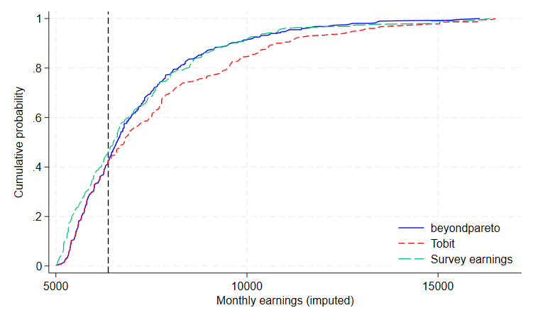
Figure 8 compares the implied top earnings shares with the target shares based on the SOEP sample. For maximum comparability, we impute for artificially censored SOEP earnings, to prevent deviations between target and imputed shares due to differing earnings concepts.
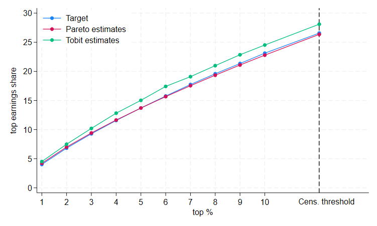
Bottom line: For the vast majority of top earnings shares,
beyondpareto’s estimates are closer to the target than the
empirical shares of the Tobit imputation. Generally, the
beyondpareto procedure slightly under-predicts, while the
Tobit imputation over-predicts. Only in the extreme part of the tail do
all three shares become, by necessity, very close.
The presented distributional approach should not be confused with individual-level imputations of censored data. The latter requires, in addition to the Pareto parameter, the assignment of a rank of to each censored observation. Due to the censoring, these ranks are unobserved. In the absence of a rank assignment of the censored observations, the calculation of top shares within the estimated tail presents the preferable option to assess the distribution of high earnings.
For further details, please consult the paper: https://doi.org/10.1515/jbnst-2024-0037